Python toolkit for simulation of the Josephson junction dynamics under the influence of external electromagnetic

In this notebook the toolkit for modeling of the Josephson junction dynamics under the influence of external radiation is presented:

• algorithm for calculation of the Josephson junctions current-voltage characteristic under the influence of external radiation;

• algorithm for calculation of the amplitude dependence of Shapiro step width;

• algorithm for calculation of the amplitude dependence of Shapiro step width in parallel regime using the Joblib library;

• results of analysis of the parallel computing efficiency.

The study is based on papers:

1. Josephson B.D. Possible new effects in superconductive tunnelling // Physics Letters - 1962. - V. 1, no. 7. - P. 251-253.

2. Shapiro S. Josephson currents in superconducting tunneling: The effect of microwavesand other observations // Phys. Rev. Lett. - 1963. - V. 11, no. 2. - P.80-82.

3. McCumber D.E. Effect of ac Impedance on dc Voltage-Current Characteristics of Superconductor Weak-Link Junctions // Journal of Applied Physics - 1968. - V. 39, no. 7. - P.3113-3118.

1. Model description

Josephson effect and Josephson junction

The coupling of two superconducting layers through a thin layer of non-superconducting barrier forms a structure called a Josephson junction (in honor of the British scientist Brian Josephson). When an electric current is passed through a Josephson junction (JJ), depending on the current value, a stationary and non-stationary Josephson effect is observed.

Stationary Josephson effect. When a current passes below the critical value \((I<I_{c})\), there is no voltage in the junction and a superconducting current flows through the junction. This current is proportional to the sine of the phase difference of the order parameters of the superconductor layers:

\( \begin{eqnarray} I_{s}=I_{c}\sin\varphi. \label{eq1} \tag{1} \end{eqnarray} \)

Non-stationary Josephson effect. When the current increases above the critical value \((I>I_{c})\), an AC voltage appears in the JJ, which is proportional to the time derivative of the phase difference

\( \begin{eqnarray} V=\frac{\hbar}{2e}\frac{d\varphi}{dt}. \label{eq2} \tag{2} \end{eqnarray} \)

System of equations for description of the JJ’s dynamics:

The dynamics of the JJ can be described within the framework of the RCSJ model (Resitively Capasitevily Shunted Junction) [3]. Within this model, the JJ is modeled as a parallel connection of a capacitor, resistor and superconductor:

A displacement current flows through the capacitor \(\displaystyle I_{disp}=C\frac{dV}{dt}\), through the resistor - quasiparticle current \(\displaystyle I_{qp}=\frac{V}{R}\) and through the superconductor Josephson (superconducting) current \(I_{s}=I_{c}\sin\varphi\).

The total current passing through the system is equal to the sum of the above mentioned currents

\( \begin{eqnarray} I=C\frac{dV}{dt}+\frac{V}{R}+I_{c}\sin\varphi. \label{eq3} \tag{3} \end{eqnarray} \)

Using (2) and (3) in normalized quantities, we can write a coupled system of differential equations with respect to \(V\) and \(\varphi\)

\( \begin{eqnarray} \begin{cases} \displaystyle \frac{dV}{dt} = I-\beta V-\sin\varphi,\\ \displaystyle \frac{d\varphi}{dt}=V, \end{cases} \label{eq4} \tag{4} \end{eqnarray} \)

where \(\displaystyle \beta=\frac{\hbar \omega_{p}}{2 e I_{c}R}\) - dissipation parameter, \(\displaystyle\omega_{p}=\sqrt{\frac{2 e I_{c}}{\hbar C}}\) - plasma frequency. In the system of equations (\ref{eq4}) time is normalized to \(\omega_{p}\), voltage is normalized to \(\displaystyle V_{0}=\frac{\hbar \omega_{p}}{2 e}\) and the current is normalized to \(I_{c}\).

The influence of external radiation on the JJ’s dynamics and Shapiro step

Under the influence of external radiation, in case of multiple Josephson frequency to the external radiation frequency a time-independent superconducting current arises as a result of frequency locking of Josephson oscillation by the external radiation. This superconducting current appears on the current-voltage characteristic (I-V characteristic) as a constant voltage step, called the Shapiro step [2]. The width of the Shapiro step depends on the frequency and amplitude of the external radiation.

In order to modeling of this phenomena, in the system of equations of the RCSJ model should be taken into account additional AC current \(I_{R}\), created by the external radiation with amplitude \(A\) and frequency \(\omega\), i.e. \(I_{R}=A\sin(\omega t)\).

The calculation algorithm of current voltage characteristic is based on solution of system of equations at a fixed current value with a choosen step. We should note that during the solution of the system of equations for each current value, the time changes from zero to \(T_{\max}\). In this case, if the equations depend explicitly on time, then it becomes necessary to realise continuously changing of time for all current intervals.

In order to realise it we need to count the number of current steps and multiply by \(T_{\max}\) and add reults to the time value. This complexity can be leveled by adding to the system of equations an additional equation like \(du/dt=\omega\). Then it is only necessary to transfer the initial condition to the next current step, which simplifies the calculation process.

Thus, the final form of the system of equations takes the form:

\( \begin{eqnarray} \begin{cases} \displaystyle \frac{dV}{dt} = I+A\sin(u)-\beta V-\sin\varphi,\\ \displaystyle \frac{d\varphi}{dt}=V,\\ \displaystyle \frac{du}{dt}=\omega. \end{cases} \label{eq5} \tag{5} \end{eqnarray} \)

Model parameters:

• \(\beta\) - dissipation parameter;

• \(A\) - external radiation amplitude;

• \(V\) - voltage;

• \(I\) - external current;

• \(\omega\) - radiation frequency;

• \(\varphi\) - phase difference.

Formulation of the problem:

Calculate the current-voltage characteristic of a Josephson junction under the influence of external radiation and plot it.

2. Calculation of current-voltage characteristics

Algorithm for calculation of the current-voltage characteristic:

1. We set the values of the model parameters, numerical calculation parameters and initial conditions.

2. We numerically solve the Cauchy problem for a system of ordinary differential equations (5), (for example, by the fourth order Runge-Kutta method) for fixed value of current \(I\), and find the time dependence of the phase difference \(\varphi(t)\) and voltage \(V(t)\).

3. We average the resulting \(V(t)\) by time:

\( \displaystyle <V>=\frac{1}{T_{\max}-T_{\min}}\int\limits_{T_{\min}}^{T_{\max}}V(t)dt \)

As a result, we obtain the voltage value for a given value of current, i.e. we obtain one point on the current-voltage characteristic.

4. We change the current value to \(\delta I\) and repeat step 2, using \(\varphi(T_{\max})\) and \(V(T_{\max})\) as the initial condition from the previos value of current and for the resulting \(V(t)\) perform step 3 to find the average voltage value.

5. We carry out calculations until \(I_{\max}\).

6. We carry out calculations by decreasing the current value \(I\) from \(I_{\max}\) to zero.

Now, let’s move directly to the implementation of this algorithm.

Importing libraries

import numpy as np
import matplotlib.pyplot as plt
from scipy.integrate import solve_ivp
from functools import partial
from scipy.integrate import odeint
import time

import seaborn as sns
sns.set()
sns.set(style="whitegrid")

%matplotlib inline

Determination of the right sides of the equations

# Function for determination of right side of equation
def shortjj(t, S, beta, Iext, A, omega):
    ''' Defines the right-hand sides of an ODE system (5),
        beta, A, omega - model parameters,
        S=[phi,V,u] - required solution '''
    ph = S[0]
    V = S[1]
    u = S[2]
    dph = V
    dV = Iext - np.sin(ph) - beta * V + A * np.sin(u)
    du = omega
    dS = [dph, dV, du]
    return dS

Calculation of the time dependence of voltage

We define a function for calculation of the time dependence of voltage and phase at a fixed value of the external current, which, using the initial conditions, values of model parameters and numerical calculations, returns the corresponding time dependences.

We define a function for the numerical solution of the Cauchy problem

def jjsolution(s0, Iext, beta, A, omega, nt, t0, deltat):
    ''' Numerical solution of the Cauchy problem for an ODE system (5),
        beta, A, omega - model parameters,
        nt - number of points in time at which the solution is located,
        t0 - initial time value,
        deltat - time step,
        Iext - external current value,
        s0=[phi0, V0, u0] - initial conditions,
        output: [phtime, Vtime, utime] - arrays of calculated time dependencies for phase, voltage and the introduced auxiliary function u '''
    f = partial(shortjj, beta=beta, Iext=Iext, A=A, omega=omega)
    t_e = np.linspace(t0, nt*deltat, nt)
    sol_1 = solve_ivp(f, [t0, nt*deltat], s0, t_eval=t_e, method='RK45',
                      rtol=1e-8, atol=1e-8)
    phtime = sol_1.y[0]
    Vtime = sol_1.y[1]
    utime = sol_1.y[2]
    return [phtime, Vtime, utime]

In order to check the correctness of the implemented computational scheme, we will find the time dependences of voltage in two modes:

1. in a state with zero average voltage,

2. in finite average voltage state.

According to the physics of the Josephson junction, as the result we should get in the first case a damped voltage, and in the second case voltage oscillation with a finite average value.

To do this, it is necessary to select the current values at which the implementation of such solutions is possible (For example \(I=0.4\)) and we need to solve a system of equations with different initial conditions for voltage (For example, \(V=0\) for first case and \(V=3\) for second one). For simplicity, we consider the case without external radiation, i.e.. \(A=0\).

Model parameters

beta = 0.2  # Dissipation parameter
A = 0  # External radiation amplitude
omega = 2 # External radiation frequency

Numerical parameters

Tmax = 100 # Maximum time value
deltat = 0.05  # time step
t0 = 0
nt = int(Tmax/deltat)

1. Solution for zero average voltage state

Iext = 0.4  # External current value
V0 = 0  # Voltage value at the initial time

time_array = np.linspace(0, Tmax, num=nt)
s0 = np.array([0, V0, 0])
res = jjsolution(s0, Iext, beta, A, omega, nt, t0, deltat)
Vtime = res[1]

We draw a time dependence \(V(t)\)

fig = plt.figure(figsize=(8, 6))
plt.plot(time_array, Vtime, label='Time dependence', linewidth=3.0)
plt.xlabel('Time', size=12)
plt.ylabel('V', size=12)
plt.legend(loc='upper right')
plt.show()

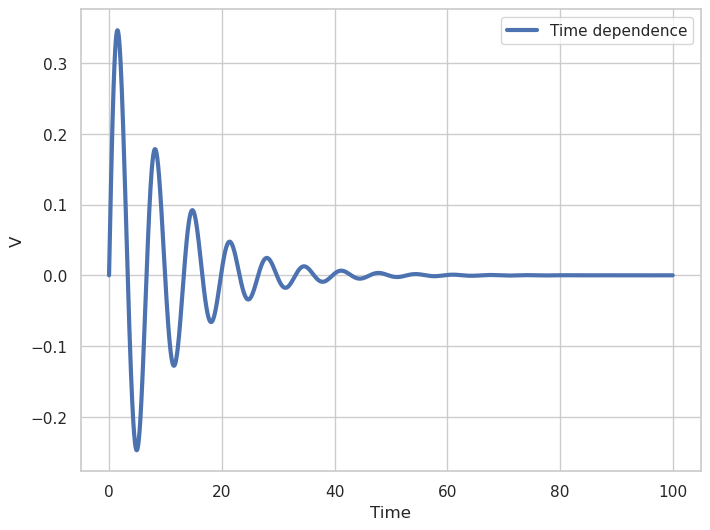
Fig. 1. Voltage versus time plot with zero average voltage

To save the resulting Figure, we can use Matplotlib library method:

fig.savefig('Vtime1.png')

To save calculation results to a file, we can use NumPy library method:

time_dep = np.column_stack((time_array, Vtime))
np.savetxt('Vtime1.dat', time_dep)

As it was noted above, according to JJ physics, the voltage value should tend to zero. As can be seen from Fig. 1, at the beginning of the integration interval, the voltage value, oscillating, tends to zero and stabilizes starting from time \(T_{min}=60\). Therefore, further for averaging it is necessary to take this fact into account, i.e. we need to calculate the average value after the stabilization of the solution.

2. Solution for the finite average voltage state

Iext = 0.4  # External current value
V0 = 3  # Voltage value at the initial time

time_array = np.linspace(0, Tmax, num=nt)
s0 = np.array([0, V0, 0])
res = jjsolution(s0, Iext, beta, A, omega, nt, t0, deltat)
Vtime = res[1]

Let’s build a time dependence graph \(V(t)\)

fig = plt.figure(figsize=(8, 6))
plt.plot(time_array, Vtime, label='Time dependence', linewidth=3.0)
plt.xlabel('Time', size=12)
plt.ylabel('V', size=12)
plt.legend(loc='upper right')
plt.show()

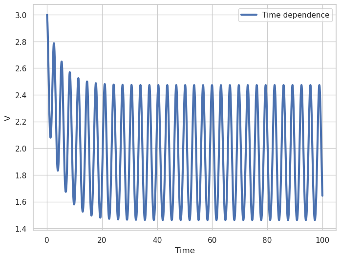
Fig. 2. Voltage versus time plot with final voltage

At this stage, the step 2 of the algorithm for calculation of the current-voltage characteristic has been implemented. Now we define a function for averaging of voltage \(V(t)\) and calculation of one point of the current-voltage characteristic.

We average the calculated voltage values at a given external current value

We set a function for averaging the time dependence of voltage

def averageV(ntmin, nt, deltat, V):
    intV = 0
    for i in range(ntmin, nt):
        intV += V[i]*deltat
    Vav = intV/((nt-ntmin)*deltat)
    return Vav

We set a function for calculation of one point of the current-voltage characteristic

def cvcpoint(s0, Iext, beta, A, omega, nt, t0, ntmin, deltat):
    solution = jjsolution(s0, Iext, beta, A, omega, nt, t0, deltat)
    phtime = solution[0]
    Vtime = solution[1]
    utime = solution[2]
    s0 = np.array([phtime[nt-1], Vtime[nt-1], utime[nt-1]])
    Vav = averageV(ntmin, nt, deltat, Vtime)
    return [Vav, s0]

Calculation of the current-voltage characteristic

Set the parameter values for calculation of the current-voltage characteristic

We note that in case of calculation, it is necessary to approve time characteristics with the period of external radiation in order to avoid the accumulation of errors during averaging. To do this, we need to calculate the period of external radiation \(T=2\pi/\omega\). From the above demonstrated time dependencies it is clear that the solution stabilizes after \(T_{\min}=60\) (for \(\omega=2\)), this corresponds approximately \(T_{\min}=20T\) (start of the averaging interval). In order to calculate the current-voltage characteristic, if we select a time interval \(T_{\max}=250\) this will correspond approximately \(T_{\max} = 80T\) (maximum time value) and, respectively, the time step \(\Delta t=T/50\).

T = 2 * np.pi/omega  # Period of external radiation
Tmin = 20 * T  # Beginning of the interval for integration for averaging
Tmax = 80 * T  # Maximum time value
deltat = T/50  # time step
ntmin = int(Tmin/deltat)
nt = int(Tmax/deltat)

deltaIext = 0.01
Iext = 0.0
a = 1.0
Iext_max = 1.2
A = 0.5
Vplot = []
Iplot = []
s0 = np.array([0, 0, 0])

We enter the parameter Ilimit, limiting the range of current changes to avoid calculation cycling.

Ilimit = 100

t_start = time.time()

while Iext < Ilimit:
    res = cvcpoint(s0, Iext, beta, A, omega, nt, t0, ntmin, deltat)
    Vav = res[0]
    s0 = res[1]
    Vplot.append(Vav)
    Iplot.append(Iext)
    Iext += a * deltaIext
    if(Iext > Iext_max):
        a = - 1
    if ((Iext < 0) and (a == - 1)):
        break
t_finish = time.time()

print(f'Execution time {t_finish - t_start} s')

Execution time 72.86328387260437 s

We draw the current-voltage characteristic

fig = plt.figure(figsize=(8, 6))
plt.plot(Iplot, Vplot, label='CVC', linewidth=3.0)
plt.xlabel('I', size=12)
plt.ylabel('V', size=12)
plt.legend(loc='upper left')
plt.show()

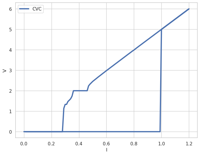
Fig. 3. Current-voltage characteristic under the external radiation with \(\omega=2\) and amplitude \(A=0.5\)

As can be seen from Fig. 3 on the current-voltage characteristic at frequency \(\omega=V=2\) a constant voltage step has formed, i.e. Shapiro step. For comparison, we can calculate the current-voltage characteristic at \(A=0\), i.e. without external radiation and make sure there is no step.

For further comparison, we should save the calculated current-voltage characteristics with external radiation in arrays Iplotrad and Vplotrad.

Iplotrad = Iplot
Vplotrad = Vplot

Calculation of current-voltage characteristics without external radiation \((A=0)\)

A = 0
a = 1
Iext = 0.0
s0 = np.array([0, 0, 0])
Vplot = []
Iplot = []

t_start = time.time()

while Iext < Ilimit:
    res = cvcpoint(s0, Iext, beta, A, omega, nt, t0, ntmin, deltat)
    Vav = res[0]
    s0 = res[1]
    Vplot.append(Vav)
    Iplot.append(Iext)
    Iext += a * deltaIext
    if(Iext > Iext_max):
        a = - 1
    if ((Iext < 0) and (a == - 1)):
        break
t_finish = time.time()
print(f'Execution time {t_finish - t_start} s')

Execution time 42.61553120613098 s

Now we can plot the obtained current-voltage characteristics with and without external radiation

fig = plt.figure(figsize=(8, 6))
plt.plot(Iplotrad, Vplotrad, label='CVC with radiation', linewidth=3.0)
plt.plot(Iplot, Vplot, label='CVC without radiation', linewidth=3.0)
plt.xlabel('I', size=12)
plt.ylabel('V', size=12)
plt.legend(loc='upper left')
plt.show()

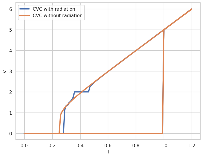
Fig. 4. Current-voltage characteristic with (\(A=0.5\)) and without (\(A=0\)) external radiation

3. Calculation of the amplitude dependence of the Shapiro step width

Algorithm for calculation of the amplitude dependence of the Shapiro step width

1. Set parameter values

2. We calculatoion of the current-voltage characteristic for a fixed amplitude of external radiation. During the calculation process, we save all values of current for which are realised the condition \(V=n_{harm}\omega\) with precision \(\varepsilon\) (\(\varepsilon>|V-n_{harm}\omega|\)) and as the difference between the maximum and minimum values from the obtained values of current, we determine the Shapiro step width. Here \(n_{harm}\) indicates the harmonic number.

3. Then increasing the amplitude value by \(\Delta A\) repeat step 2

In order to perform step 2, we will define a function that calculates the current-voltage characteristic and retuns the value of Shapiro step width.

Calculation of the amplitude dependence of the Shapiro step width

We create a function to calculate the current-voltage characteristic and find the Shapiro step width

def Shapirostepsize(A, omega, n_harm, epsilon, Ilimit,
                    beta, deltaIext, ntmin, nt, deltat):
    a = 1
    t0 = 0
    Iext = 0
    Istep_list = []
    s0 = np.array([0, 0, 0])
    getstep = False  # Variable for checking whether a step is hit
    while Iext < Ilimit:
        res = cvcpoint(s0, Iext, beta, A, omega, nt, t0, ntmin, deltat)
        Vav = res[0]
        s0 = res[1]
        # Condition for reversing the direction of the current when first hitting a step
        # Required to fully obtain a step
        if ((a == -1) and (getstep == False) and np.abs(Vav-(n_harm*omega)) < epsilon):
            a = 1
            getstep = True
            
        if ( (a==1) and (getstep==False) and np.abs(Vav-(n_harm*omega))<epsilon):
            getstep=True
        
        #Algorithm for determining the maximum and minimum current values when hitting a step
        if(np.abs(Vav-(n_harm*omega))<epsilon):
            Istep_list.append(Iext)  
        Iext+=a * deltaIext
        #The condition for changing the direction of the current when exiting the step
        if(Vav>n_harm*omega+0.05):
            a=-1
        #Condition for stopping the current cycle
        if (Vav<n_harm*omega-0.05 and a==-1):
            break
        #End of current cycle
     
    #Calculation of step width    
    Istep = max(Istep_list)-min(Istep_list)
    
    return Istep

Let us calculate the width of the Shapiro step for \(n_{harm}=1\) and \(A=1\) with precision \(\varepsilon=0.01\)

A = 1
n_harm = 1
epsilon = 0.01

t_start = time.time()
k = Shapirostepsize(A, omega, n_harm, epsilon, Ilimit,
                    beta, deltaIext, ntmin, nt, deltat)
t_finish = time.time()
print(f'Execution time {t_finish - t_start} s')
print(k)

Execution time 57.49352049827576 s
0.2300000000000002

Calculation of the amplitude dependence of the Shapiro step width in serial mode

We introduce parameters for calculation of the amplitude dependence of the Shapiro step width

• npoint - number of points in the range of amplitude values;

• Amin - minimum amplitude value;

• Amax - maximum amplitude value;

• deltaA - amplitude change step.

npoint = 160
Amin = 0.5
Amax = 40
deltaA = (Amax - Amin) / (npoint-1)
print(deltaA)

0.24842767295597484

We create an array of amplitude values for which we need to calculate the width of the Shapiro step

A_array = np.linspace(Amin, Amax, num=npoint)

Create an empty array for the Shapiro step width values

Step_array = np.zeros(npoint)

We create a function to calculate the dependence of the width of the Shapiro step on the amplitude of external radiation

def funk_ShapiroA(j, A, omega, n_harm, epsilon, Ilimit,
                    beta, deltaIext, ntmin, nt, deltat):
    A = Amin + deltaA * j

    step = Shapirostepsize(A, omega, n_harm, epsilon, Ilimit,
                    beta, deltaIext, ntmin, nt, deltat)

    return step

Calculation of the amplitude dependence of the Shapiro step width in serial mode

%%time
for i in range(0, npoint):
    Shapirostep = funk_ShapiroA(i, A, omega, n_harm, epsilon, Ilimit,
                    beta, deltaIext, ntmin, nt, deltat)
    Step_array[i] = Shapirostep

CPU times: user 3h 23min 13s, sys: 5.25 s, total: 3h 23min 18s
Wall time: 3h 23min 40s

We can plot the amplitude dependence of the Shapiro step width

fig = plt.figure(figsize=(8, 6))
plt.plot(A_array, Step_array, label='Shapiro step width', linewidth=3.0)
plt.xlabel('A', size=12)
plt.ylabel('Stepwidth', size=12)
plt.legend(loc='upper right')
plt.show()

Fig. 5. Amplitude dependence of the Shapiro step width

The calculation takes a long time, so we will carry out the calculations in parallel mode.

Parallel implementation of a computational scheme for finding the amplitude dependence of the Shapiro step width

Calculation in parallel mode using the library Joblib

To parallelize calculations by parameter \(A\) use the library functionality Joblib, which allows using the method Parallel distribute calculations over a given number of physical processor cores n_jobs. A detailed description of the library’s capabilities is presented in a separate section HLIT Jbook.

We import the necessary libraries for parallel computing

import joblib
from joblib import Parallel, delayed
import time
import os

print(f"Number of cpu: {joblib.cpu_count()}")

Number of cpu: 80

Now we can calculate the amplitude dependence of the Shapiro step width in parallel mode

def funk_parallel(j, A, omega, n_harm, epsilon, Ilimit,
                    beta, deltaIext, ntmin, nt, deltat):
    A = Amin + deltaA * j

    step = Shapirostepsize(A, omega, n_harm, epsilon, Ilimit,
                    beta, deltaIext, ntmin, nt, deltat)

    return step

t_start = time.time()
rez = Parallel(n_jobs=20)(delayed(funk_parallel)(i, A, omega, n_harm, epsilon, Ilimit,
                    beta, deltaIext, ntmin, nt, deltat) for i in range(npoint))
t_finish = time.time()
print(f'Execution time {t_finish - t_start} s')

Execution time 605.2353549003601 s

Step_array_parr = np.array(rez)

fig = plt.figure(figsize=(8, 6))
plt.plot(A_array, Step_array_parr, label='Shapiro step width',
         linewidth=3.0)
plt.xlabel('A', size=12)
plt.ylabel('Stepwidth', size=12)
plt.legend(loc='upper right')
plt.show()

Fig. 6. The amplitude dependence of the Shapiro step width